Introduction to extreme learning machine
Extreme learning machine (ELM) is a supervised learning framework that simplifies the training process of Single Hidden Layer Feedforward Neural Networks (SLFN). This framework was proposed by Huang to provide better generalization performance at extremely fast learning speed. It has been exhaustively proved that multilayer perceptron (MLP) networks with only one hidden layer can, sufficiently, approximate any continuous function giving origin to SLFNs, however, this does not guarantee optimal learning time, and generalization capabilities, and ease of implementation. SLFNs are composed of three separate layers as shown in figure below.
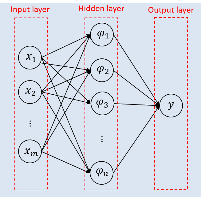
The input layer is the a set of m independent and identically distributed (i.i.d) pattern data represented by source nodes. The hidden layer is a set of n nodes where a nonlinear transform is applied to the weighted sum of the input layer data. At the output layer another weighted sum is applied, and usually this weights are updated during training as well.
Compared to SLFN-ELM, traditional supervised learning methods have shown that learning speed of feedforward networks are slower than required. Most of this traditional methods are either gradient based (e.g. backpropagation algortihm) or evolutionary algorithms. The former, could be approached as unrestricted nonlinear optimization problem; where the bottleneck lies on the existence of several local minima, with the underlying assumption of multi-modal nature of the loss function; the latter are rather global optimization problems inspired by biological evolution.
ELM’s learning algorithm randomly chooses and fixes the weights between input and hidden layer, and then analytically determines the weights of the output layer via Least Mean Square (LMS) estimators. The fact that the ELM has few parameters to be tuned lead to excel generalization capabilities. The supervised training is occurs as follows:
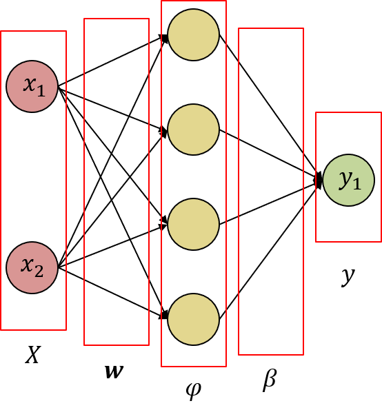
Supposed that we have a arbitrary set form by the pair {X,y}, so the SLFN_ELM could be interpreted as linear system given by:

where H is, usually called, the hidden layer output matrix, w weight vector connecting the n-th hidden node with the m-th input nodes; β is the weight vector connecting the n-th hidden layer nodes with the output layer nodes. For simplicity assume that H = H(x,w) so we have that:

For simplicity assume that H = H(x,w), that can be written as:

The input weight vector is randomly assigned and fixed. So the H matrix could be calculated by the inner product of input vector x and w given an activation function:

Since this algorithm doesn’t relies on the back propagation approach, non differential functions could be used. Then β is adjusted according to the LMS estimate which basically is the L2-norm minimization:

This is a well know linear system optimization problem whose solution It is given by least-squares estimation:

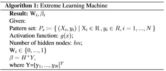
The + operator is known as the pseudo inverse or the Moore-Penrose generalized inverse of the matrix. Huang’s original algorithm is shown in the image below.
Lets code this algorith in order to make a fair test:
Activation function
def sigmoid(self, x):
        return 1/(1 + np.exp(-x))
Training function
  def train(self, Xt, Yd, nh):
        '''
        X_t: Input pattern
        Y_d: Label
        n_h: Hidden nodes
        '''
        # # Fixing random state for reproducibility
        # np.random.seed(7)
        ne = len(Xt[0])
        N = len(Yd)
        Xt = np.concatenate((Xt, np.ones((N, 1))), axis=1)
        # divide by 10 in order to improve convergence
        W = np.random.rand(ne + 1, nh)/10
        Hi = np.dot(Xt, W)
        H = self.sigmoid(Hi)
        Bi = np.dot(np.linalg.pinv(H), Yd)

        return W, Bi
Predict function
    def predict(self, Xt, W, B):
        '''
        ELM test unit for prediction
        X_t: test input pattern
        W_i: Weights vector
        B_i: Bias vector
        '''
        N = len(Xt)
        Xt = np.concatenate((Xt, np.ones((N, 1))), axis=1)
        Hi = np.dot(Xt, W)
        H = 0
        H = self.sigmoid(Hi)
        Y = np.dot(H, B)

        return Y
So first, in order to check the algorithm that we just have implemented, a simple but useful hard test is the exclusive disjunction function or XOR, which is defined as a not linearly separable function. Consider two patterns:

Shown in figure bellow is the spatial representation of XOR function for two classes that cannot be separated in a linear manner.

In order to overcome the limitations of linear separability it is possible to map this problem in a SLFN with 4 nodes in the hidden layer.
Creating an the ELM object that was created before, we have:
#pattern dataset
X = np.array([[0,0],[0,1],[1,0],[1,1]])
y = np.array([[0],[1],[1],[0]])
#Fixing random state for reproducibility
ELM = ELM()
# training step using 4 nodes in the hidden layer
W_i, B_i = ELM.train(X,y,4)
# label prediction using the calculated weigths
ELM.predict(X,W_i,B_i)
And the predicted value for each of the input patterns is printed out
array([[0.],
       [1.],
       [1.],
       [0.]])
Check out the ELM repo for more info.