Probabilistic neural networks in a nutshell
Probabilistic neural networks (PNN) are a type of feed-forward artificial neural network that are closely related to kernel density estimation (KDE) via Parzen-window that asymptotically approaches to Bayes optimal risk minimization. This technique is widely used to estimate class-conditional densities (also known as likelihood) in machine learning tasks such as supervised learning.

The neural network that was introduced by Specht is composed by four layers:
- Input layer: Features of data points (or observations)
- Pattern layer: Calculation of the class-conditional PDF
- Summation layer: Summation of the inter-class patterns
- Output layer: Hypothesis testing with the maximum a posteriori probability (MAP)
In order to understand the back-bone mechanism of the PNN, one have to look back to Bayes theorem. Suppose that the goal is to is to built a Bayes classifier, where X and Θ are independent and identically distributed (i.i.d) random variables (r.v).
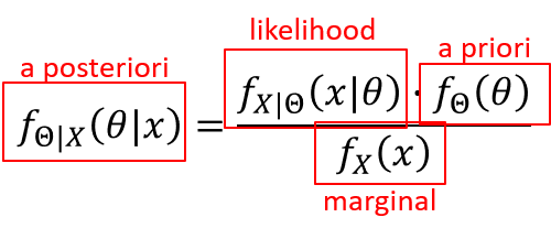
whereas finding the likelihood probability density function (PDF) could be a challenging problem; using Parzen-window method to calculate it, tackles down this problem in a elegant and reliable way. Therefore, if the parameters of the likelihood PDF are known, it will be easy to infere the posterior probability.
The Parzen-window is, basically, a non-parametric method to estimate the PDF for a specific observation given a data set; conversely, this doesn’t require prior knowledge about the underlying distribution. This window has a weighting funtion Φ and smoothing funtion h(n). (For further knowledge about KDE visit sebastian raschka webpage)

Using the normal distribution as weighting funtion lead us to the following equation, normalized by the total number of class conditional observations.

In a multivariate problem Σ is a diagonal matrix that contains the covariance of each feature.

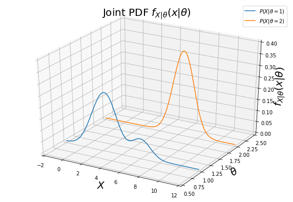
For a better understanding, take for instance a simple univariate case study. Suppose that X is an i.i.d random variable that is composed by a set of binomial class data. Assume that σ=1, and a unclassified observation x=3.


Let Θ be a Bernoulli random variable that indicates the binomial class hypotheses, and let P(Θ) equaly likely. Under the hypothesis Θ=1, the random variable X has a PDF defined by:

Under the alternative hypothesis Θ=2, X has a normal distribution with mean 2 and variance 1.

Therefore, a solution of x, that satisfies the boundary condition, can be found numerically. This is an optimal solution, that minimizes the misclassification rate. A proxy visual representation of the the hypothesis test of class conditional funtions is shown bellow.

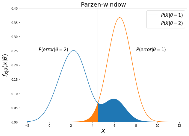
The decision boundary of the PNN is given by:

The figure bellow shows the decision boundary and the error conditional probability (shaded region).
Finally, having observed x, is choosen an estimate that maximizes the posterior PDF ovel all Θ, via MAP.

Given the MAP estimator, the outcome will be y2(x)=0.0011 < 0.2103 = y1(x), thus, the observation will be classified as Θ=1.
In order to compare with other machine learning algorithms, was created a python class that matches the structure of SciKit Learn algorithms. Using the default benchmark composed by 3 synthetic datasets was made a comparisson with a Gaussian process and a Nearest Neighbors classifiers.The image bellow shows the results achieved measured by the accuracy metric.
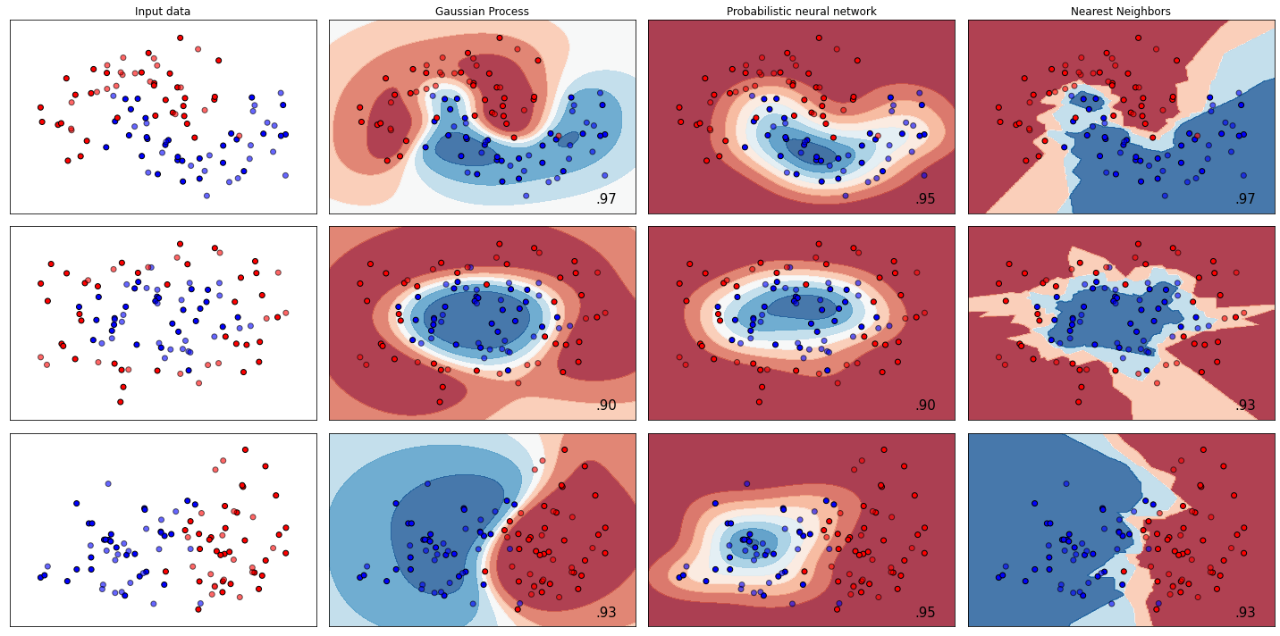
Check out the PNN repo for more info.