Processing medical images for deep learning applications

Image preprocessing is a fundamental step in any deep learning model building process, especially when it comes to medical images that we heavily rely on such as X-ray and computer tomography(CT). Whether you are new to image processing or you have some experience, this is an overview of the challenges that may be faced when dealing with such images and how to overcome some of the common pitfalls. From reading raw DICOM files and anonymizing them to assembly tensor data of the input layer or even preparing data for radiomics analysis, this post uses SimpleITK to achieve such tasks. SimpleITK is a procedural ITK’s wrapper for python language that has many bindings from ITK popular package.

Intro

Several machine learning and deep learning applications using medical images still rely on some technologies such as X-ray and computed tomography (CT) for disease diagnosis and prognosis. Building a successful data set using these images depends on image quality aspects such as signal-to noise ratio (SNR) and intensity homogeneities to perform in a reasonable manner. Dealing with inhomengities is a key aspect, since homogeneous datasets could perform better during the training stage of the model. Another important aspect is the link between existing health care systems (e.g. PACS) and medical applications that should be in compliance with privacy regulations.

Most of medical images are in DICOM (Digital Imaging and Communications in Medicine) format, that are a combination of metadata regarding clinical and pixel data. The former comes in tuple like tags denoted by 2 hexadecimal numbers, for instance: (0010,0020) which contains Patient ID; the later contains pixel spacing and size (usually 512 x 512).

The following image is an overview of a typical CT pre process pipeline for deep learning aplications. It assumes, and for the sake of protected data that the original file have been anonymized and goes all the way to creating of the input tensor.

Reading DICOM files

ITK package offers a comprehensive tool for reading DICOM data in a procedural fashion. The following code snippet shows how to read a CT scan and if everything went well it displays series description from the metadata. For better understanding of DICOM fields check this resource.

series_reader = sitk.ImageSeriesReader()
series_reader.SetFileNames(<path_to_series>)
series_reader.MetaDataDictionaryArrayUpdateOn()
series_reader.LoadPrivateTagsOn()
try:
  ct_scan = series_reader.Execute()
except:
  print("some reading error!")
  pass
else:
  series_description = series_reader.GetMetaData(0, '0008|103e')
  print(series_description)

Not very often is nedded to work with DICOM files, that is aheavy weighted file format, so is desirable to work with with something much more light weight. NIfTI(Neuroimaging Informatics Technology Initiative) format is a good candidate for the joba and it can be read by nearly all medical imaging platforms (e.g mango). Using the snippet before, once the DICOM file is read, it can be saved as *.nii.gz.

sitk.WriteImage(ct_scan,<output_path>+'ct_scan.nii.gz')

Anonymization

Anonymizing and de-identifying patient data should be the first step in any medical application pipeline, since according to the newest LGP regulations, sensible data should be avoided when sharing datasets among the internet. These privacy regulations must be in compliance with organizations such as HIPAA in the US and the PIPEDA in Canada. Recently the Radiological Society of North America(RSNA) made available an anonymization tool for such purpose.

Windowing

Usually CT data is restricted to −1024 and 3071 range in Hounsfield Units (HU). Values less than −1024 HU are commonly found due to areas of the image outside the field of view (FOV) of the scanner. The first step towards enhancing the image according to the specific needs, would be to Winsorize the data to the [−1024, 3071] range, or whatever is your purpose. The following table shows the most common ranges for some anatomical regions of the body.

The following comparisson uses mango for reading the chest CT scan. The image on the left has a HU window of [-1000,400], and the right has a HU range of [-400,600]. Diffent ranges enhances some anatomic structures of the lung parenchyma.

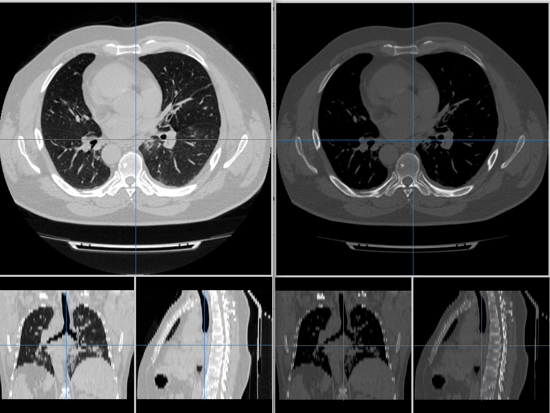
Let’s take for instance …

def hounsfield_to_cormack(self, image):
        '''
        Conversion formula suggested by Chris Rorden
        in matlab's clinical toolbox
        https://www.nitrc.org/projects/clinicaltbx/
        '''
        img_data = sitk.GetArrayFromImage(image)
        t = img_data.flatten()
        t1 = np.zeros(t.size)
        t1[np.where(t>100)] = t[np.where(t > 100)]+3000
        t1[np.where(np.logical_and(t >= -1000, t <= -100))]=t[np.where(np.logical_and(t >= -1000,t <= -100))]+1000
        t1[np.where(np.logical_and(t >= -99, t <= 100))]=(t[np.where(np.logical_and(t >= -99, t <= 100))]+99)*11+911
        trans_img = t1.reshape(img_data.shape)

        res_img = sitk.GetImageFromArray(trans_img)
        res_img.CopyInformation(image)

        return res_img

Resample

def resampleImage(image):
        '''
        Resample funtion for deep learning preprocess purpose
        image: ITK's compatible format image
        reference_size: downsampled size in vector like format (i.e. [sx, sy, sz])
        '''
        #TODO: add loggin capabilities
        original_CT = image
        # NIfTi(RAS) to ITK(LPS) 
        original_CT = sitk.DICOMOrient(original_CT, 'LPS')
        dimension = original_CT.GetDimension()
        reference_physical_size = np.zeros(original_CT.GetDimension())
        reference_physical_size[:] = [(sz-1)*spc if sz*spc>max_  else max_ for sz,spc,max_ in zip(original_CT.GetSize(), original_CT.GetSpacing(), reference_physical_size)]
        
        reference_origin = original_CT.GetOrigin()
        reference_direction = original_CT.GetDirection()
        #FIXME: Looks like the downsampled image is mirrored over the y axis
    #     reference_direction = [1.,0.,0.,0.,1.,0.,0.,0.,1.]
        reference_size = image_size
        print(reference_size)
        reference_spacing = [ phys_sz/(sz-1) for sz,phys_sz in zip(reference_size, reference_physical_size) ]

        reference_image = sitk.Image(reference_size, original_CT.GetPixelIDValue())
        reference_image.SetOrigin(reference_origin)
        reference_image.SetSpacing(reference_spacing)
        reference_image.SetDirection(reference_direction)

        reference_center = np.array(reference_image.TransformContinuousIndexToPhysicalPoint(np.array(reference_image.GetSize())/2.0))
        
        transform = sitk.AffineTransform(dimension)
        transform.SetMatrix(original_CT.GetDirection())
        # transform.SetMatrix([1,0,0,0,-1,0,0,0,1])
        transform.SetTranslation(np.array(original_CT.GetOrigin()) - reference_origin)
        # Modify the transformation to align the centers of the original and reference image instead of their origins.
        centering_transform = sitk.TranslationTransform(dimension)
        img_center = np.array(original_CT.TransformContinuousIndexToPhysicalPoint(np.array(original_CT.GetSize())/2.0))
        centering_transform.SetOffset(np.array(transform.GetInverse().TransformPoint(img_center) - reference_center))
        centered_transform = sitk.CompositeTransform([transform, centering_transform])

        # sitk.Show(sitk.Resample(original_CT, reference_image, centered_transform, sitk.sitkLinear, 0.0))
        
        return sitk.Resample(original_CT, reference_image, centered_transform, sitk.sitkLinear, 0.0)

Pseudo color converison

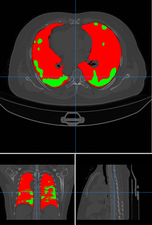
Usually consolidated deep learning architectures for medical images have multiband like tensors that normally rely on RGB images. When using gray scale images (or even Hounsfield scale) comes in handy the use of pseudo color techniques that may enhance the target features within. This works whether you are using channels_first(NCHW) or channels_last (NHWC) conventions in TensorFlow for instance. The pseudocode (image below) shows how this process works.

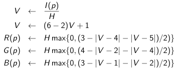
The code bellow implements this idea creating an multi band image in YCbCr color space for deep learning purposes.

def grey_to_color(image):
    """
    Converts an image array from grayscale (3 stacked channels) to YCbCr
    
    image:  gray scale image(w, h, 3)
  
    """
    R_channel = []
    G_channel = []
    B_channel = []
    ## Create LUT Red-Blue table
    H = pow(2,8)
    for elt in range(0,H):
        # lut_x = np.append(lut_x, np.floor(GrayScaleToBlueToRedColor(elt,255)).astype('uint8'), axis=0)
        R,G,B = np.floor(GrayScaleToBlueToRedColor(elt,H-1)).astype('uint8')
        R_channel.append(R)
        G_channel.append(G)
        B_channel.append(B)

    R_channel = np.asarray(R_channel)
    G_channel = np.asarray(G_channel)
    B_channel = np.asarray(B_channel)

    lut = np.dstack((B_channel, G_channel, R_channel))
    image = cv2.LUT(image, lut)
    image = cv2.cvtColor(image, cv2.COLOR_BGR2YCrCb)
    
    return image